
Building Dynamic Charts with Named Ranges
This article dives deeper into two methods of creating a dynamic chart. The methods include: (i) Named Ranges with OFFSET and (ii) Excel 365’s new FILTER function. This new FILTER function makes chart automation much easier, allowing you to create powerful automation with much less complexity.
In one of our other resources, we shared five important tips on how you can automate your charts. This article builds on the first tip and demonstrates the power of data automation for charting. [These are advanced techniques with many steps, so we have included a sample worksheet that you can download to see the formulas and complete setup.]
1. Using the OFFSET formula and Named Ranges:
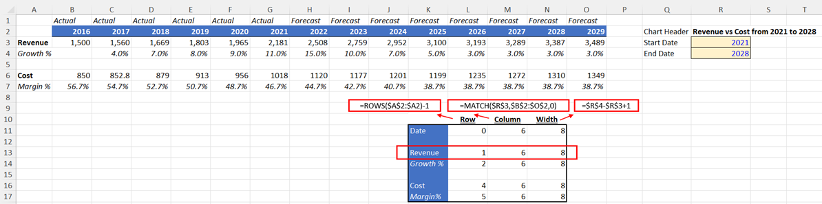
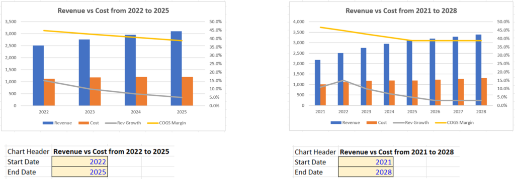
To construct our dynamic chart, we use an example of historical and estimated Revenues and Costs as outlined below. We’ve added three placeholders, including “Chart Header” to customize chart title using dynamic text, “Start Date” and “End Date” parameters. This helps us define our data range for the chart and provide control to the user.
To construct our dynamic array, we can use the OFFSET function. However, since charts cannot use OFFSET functions as inputs directly, we need to use Named Ranges. This allows us to create an array that is defined by the OFFSET function. Then use this Named Range (thus a “Dynamic” Named Range) in our chart formula (i.e., to reference the array calculated by the OFFSET). Our goal is to create an array that automatically captures data between the Start and End Date when the inputs change.
To assign Named Ranges to our data sets, first we need to go to Formulas -> Name Manager (steps 1 & 2). On the pop-up window click the “New…” button on the top left corner (step 3) as illustrated below.
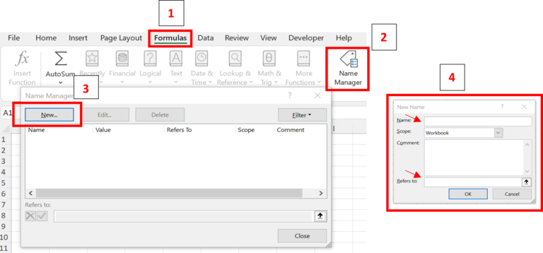
Using the menu shown in step 4, we then provide a name to our data array (remember it cannot contain spaces and must start with a letter), and insert our OFFSET function in the “Refers to:” box with the following syntax:
=OFFSET(reference, rows, cols, [height], [width]).
We first assign a reference point above and to the left of our data, which we select as $A$2, and in the next two arguments define the number of rows and columns away from our reference cell to locate the start of our data set.
The diagram below shows the coordinates for our OFFSET formula and the calculations that generate the required inputs that capture the desired array. We want to move down one row for Revenue, so we enter “=ROWS($A$2:$A3)-1” for the second argument (rows). Notice that we unlocked “$A3” so we can easily copy and paste the formula for other data sets (Date, Growth %, Cost, Margin %). For our third argument (cols for “columns”) we use the Match function “=MATCH($R$3,$B$2:$O$2,0)” to return the location of our starting date in our date set from columns B to O. With the last two inputs, given we only want one row of data so we can enter 1 for height (or simply not enter any values) followed by a comma. Finally the fifth argument (width), we calculate the difference between our end date and start date +1, or (=$R$4-$R$3+1).
To make the OFFSET formula simpler to apply and avoid unnecessary errors, you can create the required arguments directly in the worksheet, as shown below, and simply link to the OFFSET formula in the Name Manager. Note that you need to create inputs for each OFFSET function that will be used in each dynamic array that you need before proceeding to inserting your chart.
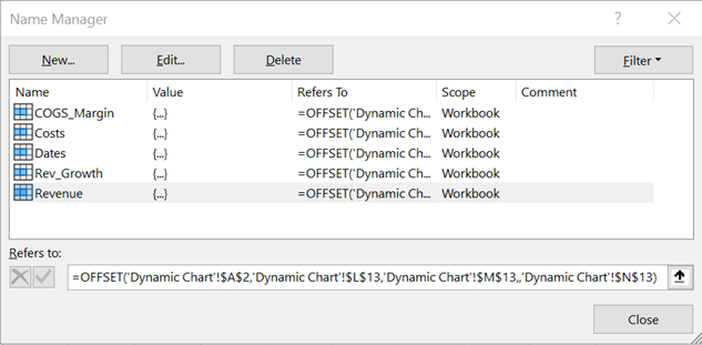
With all the Named Ranges in place, we then can create our chart and define our “Series”. Charts are objects that float above your worksheets and need both tab name and cell addresses to locate the data that they present. Therefore, when you input the Dynamic Named Range, you must include the worksheet name (in our example “Dynamic Chart”) followed by an exclamation mark in front of the name we have assigned to our dynamic range as shown below in the Edit Series menu. We enter every array in our data set to complete our chart. Additionally, we added a secondary axis to display Revenue Growth % and Cost Margin %.
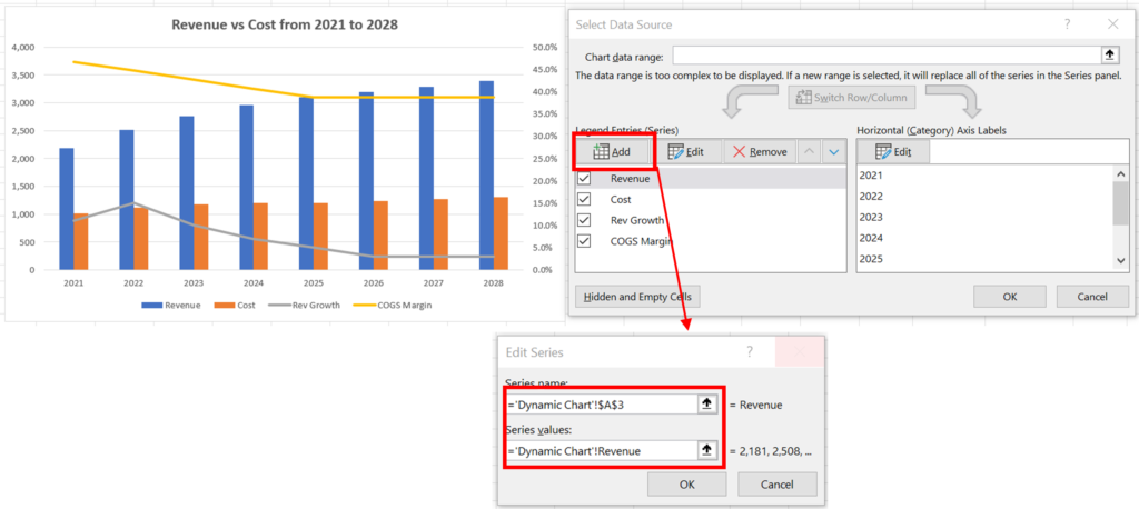
Lastly, we make our chart title text dynamic by selecting (left click) the chart title, hit “=” (you will notice an “=” sign in the formula bar), and link to cell R2. You can do the same technique for axis titles. We have also used a CONCATENATE formula “=”Revenue vs Cost from “&$R$3&” to “&$R$4” to include the start and end dates in our chart title as seen below. At this point, our chart is fully dynamic and controlled by inserting inputs for our start and end dates.
2. Using the FILTER function and Named Ranges:
Prior to Excel 365’s FILTER function, the OFFSET method was the best way to automate chart data and ranges. Now that the FILTER function is available, it is much easier to build an automated chart. If you recall from our article on Dynamic Ranges, the FILTER function creates a dynamic array based on a criteria assigned to it by the user. (click here to read more on how to use the FILTER function if you are using Excel 365).
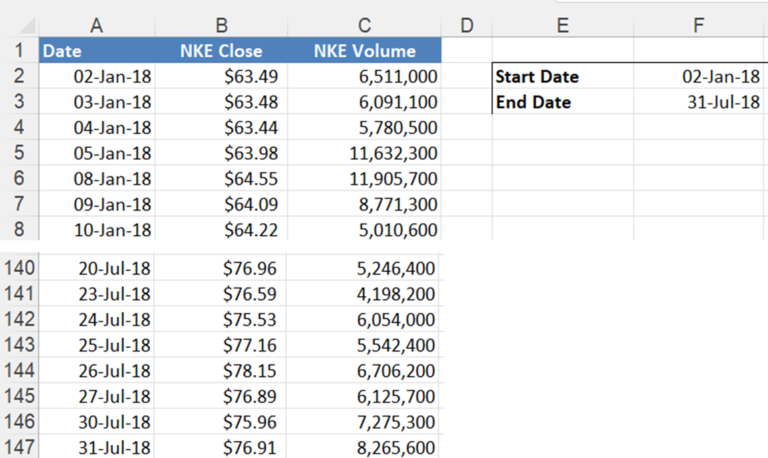
In our example below we have a sample of daily stock prices and volumes from January 2, 2018 to July 31, 2018 and we want the chart to capture the second half of the year data when we add it without adjusting our chart range manually.
Similar to our example in part 1, we added placeholders in the worksheet for our start and end dates in cells “F2” and “F3”. However, instead of manually inserting the date we can automate this by using the MIN() and MAX() functions so every time a date is added it captures it as the maximum end of the range. If you anticipate your dataset to be large, enter a large value for the range end. In our example we set our range as A2:A5000.
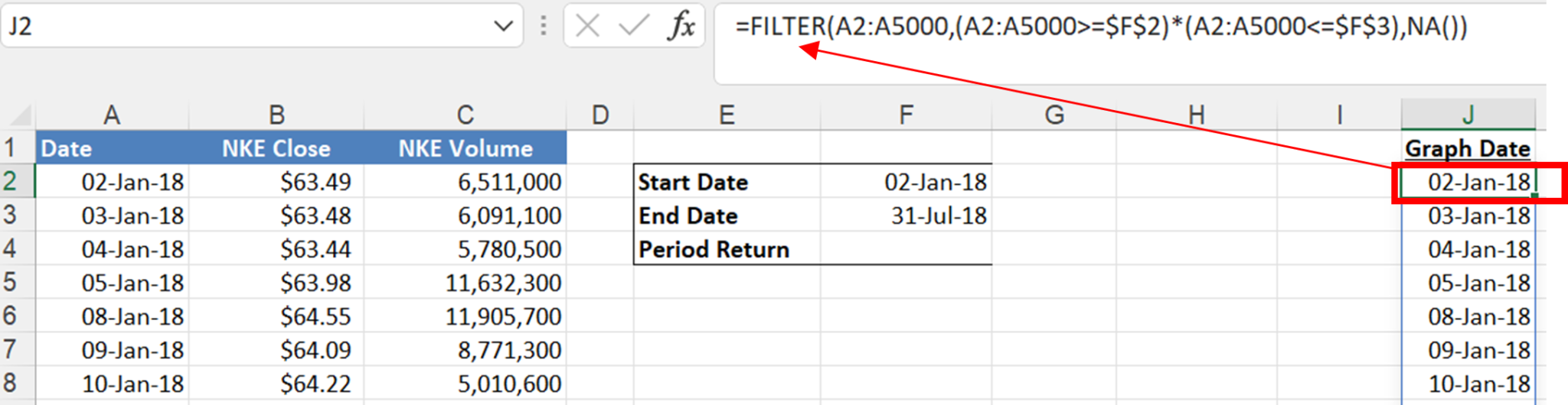
The first input argument for the FILTER function will be the range of records that we retrieve that meet our criteria (in our case B2:B5000 for Price and C2:C5000 for Volume). We need to create one array for each input for our chart so we are filtering them separately. For the second criteria, we want our filtered data set to include any cell that is “>=” to our start date, and “<=” to our end date. The last criteria which is optional, is to put an NA() function if nothing is found. A single formula will then return a range of results across a number of cells as illustrated below. We replicate the same Filter function for Price and Volume with the following formulas:
“=FILTER(B2:B5000,(A2:A5000>=$F$2)*(A2:A5000<=$F$3),NA())”
“=FILTER(C2:C5000,(A2:A5000>=$F$2)*(A2:A5000<=$F$3),NA())”
Alternatively, we could have constructed our FILTER function by retrieving all non-empty cells with
=FILTER(A2:A5000,(A2:A5000<>””),””). Or we could have retrieved all values greater than the smallest value in the range (which for ranges with blanks is zero) with
=FILTER(A2:A5000,(A2:A5000>=MIN(A1:A5000)),””).
The FILTER functions will now create spilled arrays that contain the graphing data. We have added headers above the FILTER functions to describe the values in each column. The one formula will create the entire array but make sure there are no populated cells below the columns you use as filtered ranges, otherwise you would get a #SPILL! error.
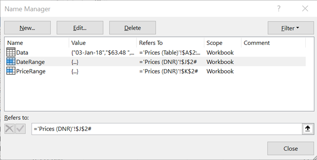
Now that we have defined our dynamic ranges, we repeat the process of using Name Manager to define our arrays (Date, Price, Volume). With the use of FILTER function, however, we only select our first cell which contains our formula for the FILTER function followed by the “#” sign. This enables Excel to automatically set the end range as the last non-empty cell in the range.
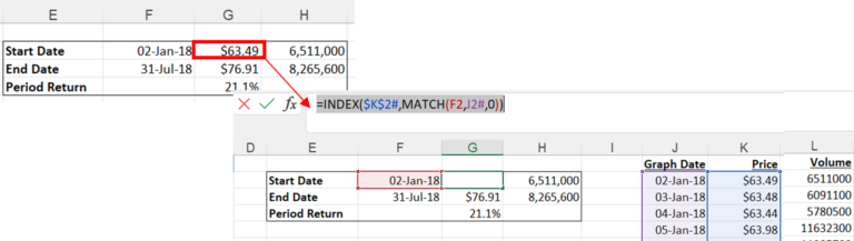
The use of filtered arrays can also be used in with an INDEX/MATCH function combination to extract the corresponding values from our graph data. For instance, to find the price at each of our start and end dates we use the INDEX/MATCH to look up the price at each date in the filtered lists. However, instead of defining our range of array, all we must do is select the first cell in the filtered list (which contains the FILTER formula) for the reference argument followed by the “#” sign, as illustrated below. Ultimately, the prices allow us to calculate an up-to-date period return as additional data is included.
We can now create our chart with the 6-month data by referring to our Named Ranges in the same way as the example in section 1. Now add the dynamic title and Period Return text box using CONCATENATE functions for each title. We can now dynamically change the date range of the chart by changing the end date. The title and return calculations update automatically.
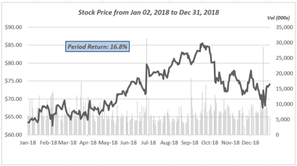
As illustrated, the FILTER function is a powerful and simple tool you can use to create your dynamic charts.
If you enjoyed reading this and want to improve your skills further, then try our Excel Best Practices Self-Study Course. You can also browse our other range of Self-Study Courses here.
Training The Street also offers a more advanced In-Person/Virtual Public Course called, Applied Excel. Where you can gain the skills needed for parsing, analyzing, and presenting information from large data sets.