Copy & Paste in Excel Using the CTRL + ENTER and SHIFT + F8 Shortcuts

When you’re working in Excel, one of the most common sequences is to fill in one cell (with say a link or a formula) and then copy and paste the same thing into adjacent cells. How many ways are there in Excel to copy and paste cells? Lots. There’s of course dragging the bottom right corner with the mouse. OK, let’s not go there, if only because that previous sentence contained the word “mouse”. Moving on, here are two great ways to speed up your copy and pasting using some lesser known shortcuts on the keyboard.

1. Copy the completed cell (CTRL +C), then select the cells (SHIFT + Arrow Keys) where you want to repeat the formula and do a Paste (CTRL + V or Enter), or Paste Special (CTRL + ALT + V) if you only want to paste some attributes of the copied cell.
2. Highlight the completed cell as well as the other destination cells and do a fill right and/or down (CTRL + R / CTRL + D) depending on the orientation of the data.

These methods are fine and certainly quicker than using the mouse. But they still involve a fair number of keystrokes. Here’s an alternative way that can speed things up even more (let’s call this option 3). Use the CTRL + ENTER shortcut – this shortcut applies the same contents or formula in all the cells you initially select. Here’s a simple example:

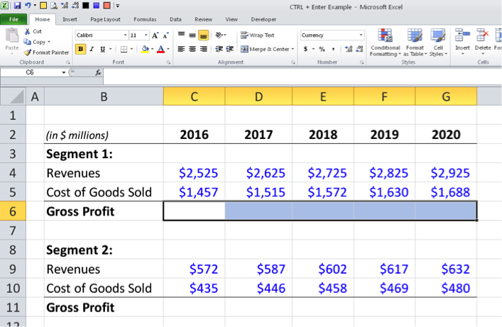
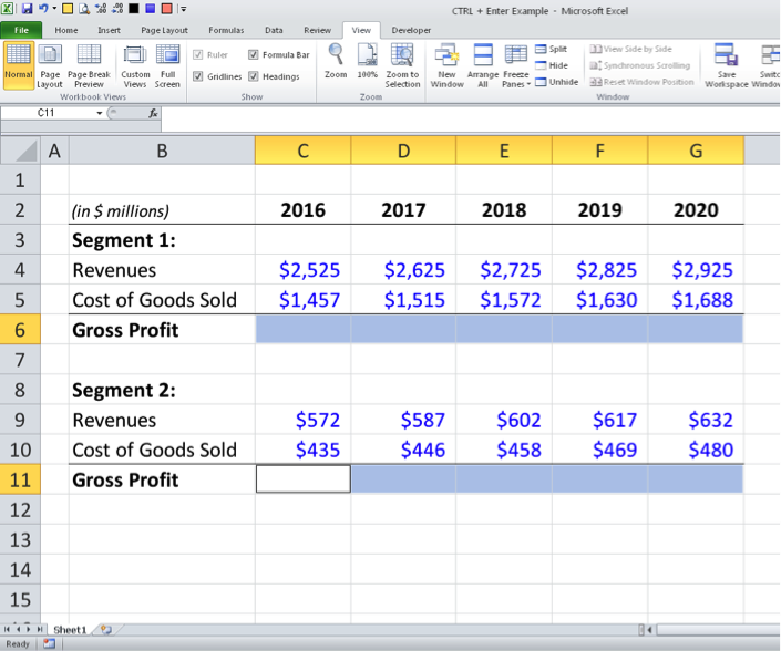
• Let’s suppose you have a simple table with revenue and cost forecasts as shown in the picture below, and you want to quickly fill in the formulas for Gross Profit in row 6.
• First, select all the cells where you want the Gross Profit calculation (C6:G6).

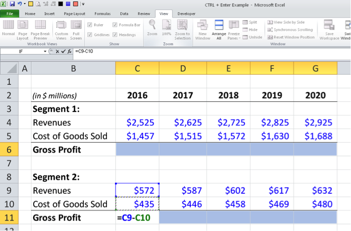
• Now start creating the formula the way you normally would (type = then up arrow twice, etc.). You’ll notice that even though multiple cells are selected, Excel will create the formula in the top left cell of the selected range (in this case, the leftmost cell C6).

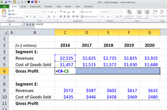
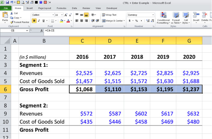
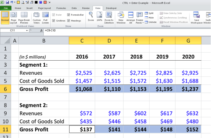
• Here’s the key step: instead of hitting ENTER the way you normally do, hit CTRL + ENTER and Excel will replicate the formula in all of the selected cells.

Pretty sweet, no? It actually saved keystrokes. We know, because we counted. Starting on cell C6, here’s a tally of the various methods and the number of keystrokes required to fill in the rest of row 6:

• Option 1: (build C6, select C6:G6, hit CTRL + R): 12 keystrokes
• Option 2: (build C6, select D6:G6, hit CTRL + V): 13 keystrokes
• Option 3: (select C6:G6, build C6, hit CTRL + ENTER): 10 keystrokes

Option 3 is 17% and 23% more efficient (ie. faster) than options 1 and 2, respectively. Part of the issue is that the first two options above require that you go back to cell C6 after you’ve initially built it.

Now let’s take this to the next level for even greater efficiency. Notice in the graphic we’ve been using, there’s another segment (Segment 2) for which we need to calculate Gross Profit. So the same formula that appeared in row 6 for Segment 1 is needed for Segment 2 in row 11 (Revenues less Cost of Goods Sold). Let’s fill in both rows 6 and 11 all at once using the SHIFT + F8 shortcut to Add to Selection before we hit CTRL + ENTER. Here are the steps:

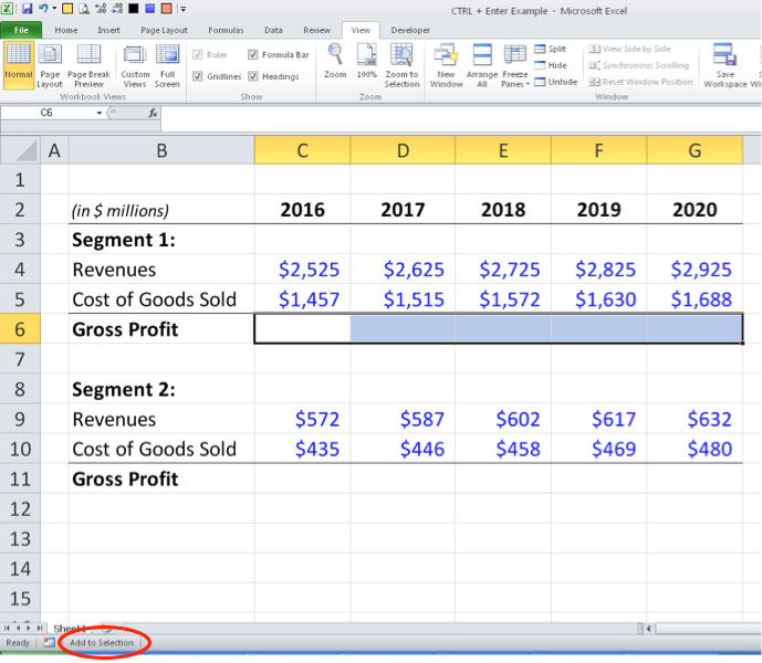
• First, select the cells in row 6 where you want Gross Profit, but before you do anything else, hit SHIFT + F8. This will allow you to use your keyboard to add cells to your selection (and you can keep repeating this step). You won’t need to use your mouse to select the additional cells. You should see “Add to Selection” in the bottom left corner of Excel, as is shown here:

• Now simply use your arrow keys to move to cell C11 and use SHIFT and the right arrow to select the rest of the range in row 11. The cells in row 6 should remain selected:

• Finally, as before, create the formula in the “active” cell (which in this case will be cell C11):

• Now hit CTRL + ENTER and voila. Excel will apply the formula logic in all the selected cells:

As you can see, using the SHIFT + F8 shortcut allows you to select multiple non-contiguous ranges of cells with the keyboard (similar to holding CTRL and selecting multiple ranges with your mouse).

It is worth mentioning one small caveat regarding using SHIFT + F8. If one of the ranges you are highlighting is a single cell, you must hit SHIFT + F8 twice in a row before highlighting the next range. (otherwise, you will lose the previously selected cells).

Experiment with this trick and we’re sure you’ll like it and use it frequently.