Creating a Dynamic Hyperlink in Excel & Use of Hyperlink Function

This article will show you the steps needed to ensure your reference cell/section does not stay static, and how to create dynamic hyperlinks in Excel.

This is the second part of our hyperlink resource on our website. You can refer back to the first part by clicking here. To summarize, we explained how you can access different worksheets or schedules within a worksheet by inserting a hyperlink. Specifically, we reviewed ways to i) insert a hyperlink; ii) make the link more user-friendly and informative; and iii) prepare a table of contents for navigation purposes.

This powerful technique has one potential shortfall: if you insert/delete columns or rows or move cells around in the spreadsheet (i.e. cut and paste), you need to ensure that your reference points are dynamic.

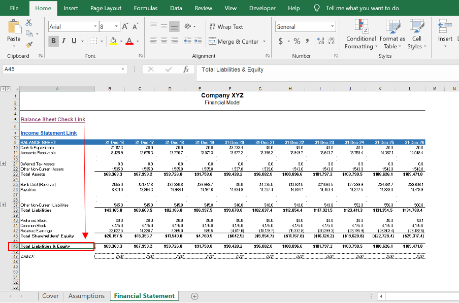
Placing a standard hyperlink is useful if your primary purpose is to navigate to other tabs or when your model is locked for adding/deleting rows and columns. Using the example below, we insert the hyperlink in cell A5 to refer to the Balance Sheet Check (cell A45).

However, with the addition of 2 rows to insert a link for the Income Statement in row A7, the hyperlink still points to cell A45 rather than the desired cell A47 as illustrated in the image below.

To solve this issue, we need to use a defined name. Defined names let you refer to a cell or to an array of cells by its name rather than specific column and row coordinates (e.g. A45).

To create a defined name, select a cell then click in the “Name Box” located in the top left corner above cell A1. You can assign any given name to the cell that does not already exist in the worksheet and press enter to name the cell. You can view all the defined names in the workbook by clicking on the dropdown menu next to the Name Box.

Note that while names are not case sensitive, there are several restrictions in assigning names to cells including the following:

• Names must begin with a letter, an underscore (_), or a backslash (\)
• Names cannot contain spaces or most punctuation characters. However, you can join letters by using an underscore (_) or a period (.)
• Names cannot conflict with cell references such as “AB1” or “W15”
• You can use single letters as names. But you can’t use “r” and “c” as they reserved for Excel shortcuts

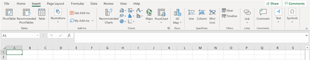
Once the defined name is created, you can use the Name Manager. You can edit the defined name as needed by going to the Formula bar tab and clicking on Name Manager. The shortcut to Name Manager is through CTRL + F3. F3 by itself launches the Paste Names menu and provides a list of all created names in the workbook. Note that the alternative method to add a New Name is by clicking “New…” box on top left when launching the Name Manager menu.

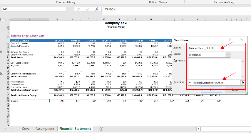
The image below shows the New Name menu and the creation of the name “BalanceSheet_CHECK” in cell A45:

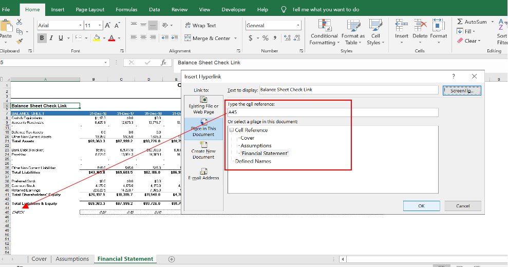
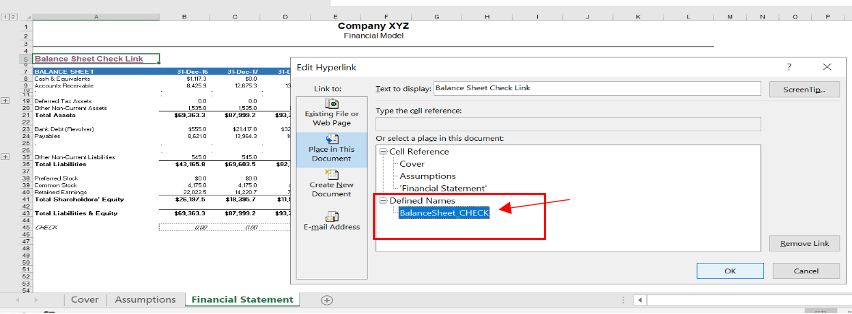
• From the cell that will have the hyperlink, in this case A5, use the keyboard shortcut to open the hyperlink menu (Ctrl + K) and the Edit Hyperlink menu will appear. You can also right click and select ”Edit Hyperlink”.
• Click the “Place in This Document” on the Left. The defined name should now appear on the menu bar under “Defined Names”. Now, you can add any extra rows between the “Balance Sheet Check” link and the balance sheet segment. Just like we did earlier, the referred cell(s) for the hyperlink is unaffected.

Hyperlinks that use a defined name also create the flexibility to copy/cut and paste the link to other worksheet(s) while keeping the reference cell(s) unchanged. This lets you copy a hyperlink into multiple locations in your model (such as a “Return to Main Menu” link).

The HYPERLINK Function Alternative:

You can also created Hyperlinks using the HYPERLINK function. This is particularly useful to link to a list of locations/need the hyperlink to refer to an Excel Table range.

To insert a HYPERLINK function, select the intended cell you’d like to contain the hyperlink and insert the following syntax:

=HYPERLINK(link_location,[friendly_name])

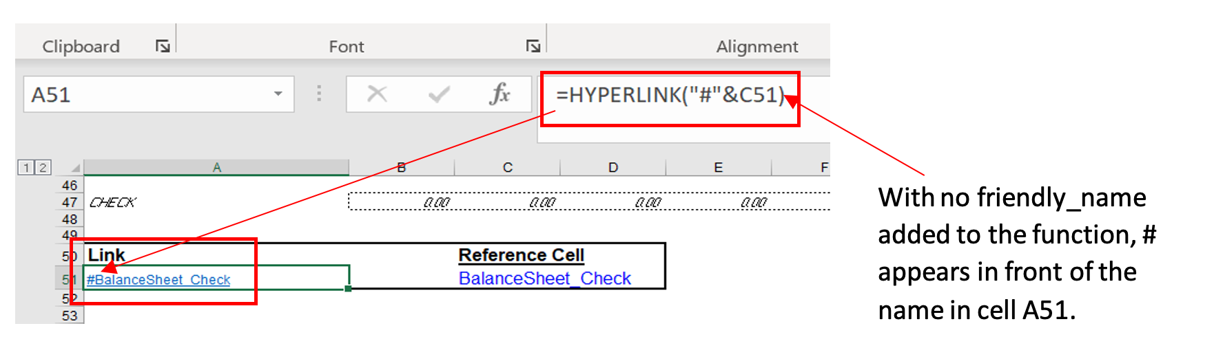
The first argument should include the targeted reference cell or external link (Email address / URL, document file path). The second argument is the name that is the displayed name given to the hyperlink. The latter is optional and if not inserted, the cell will display the link location as the name of the hyperlink. The format for the link location is, however, slightly different if you would like to refer to a defined name that you have assigned to a cell or a table, for instance. You need to add a hashtag (#) in front of the defined name, as illustrated in the syntax below. This can be followed by the assigned name, with each input embedded in double quotation marks (“ ”). Be sure to add the defined name as the friendly_name argument so that the # won’t appear in front of the name of the hyperlink.

=HYPERLINK(“#Defined Name”,[friendly_name])

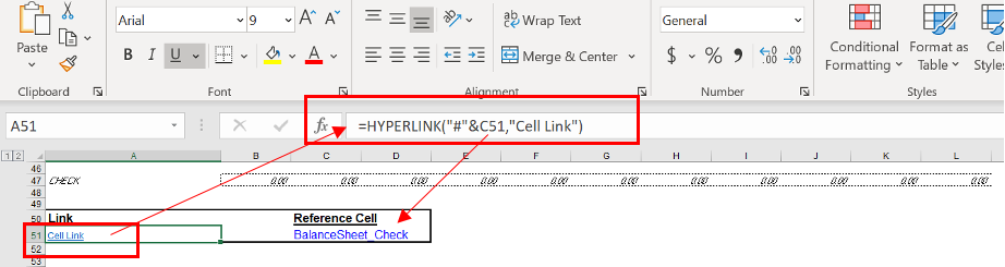
In the example below, we have inserted the assigned defined name for Balance Sheet Check in cell C51. We’ve used it as our link location in the first part of the HYPERLINK function. This is the equivalent of using the defined name directly in the function in the following format:

=HYPERLINK(“#”&”BalanceSheet_Check”,”Cell Link”)

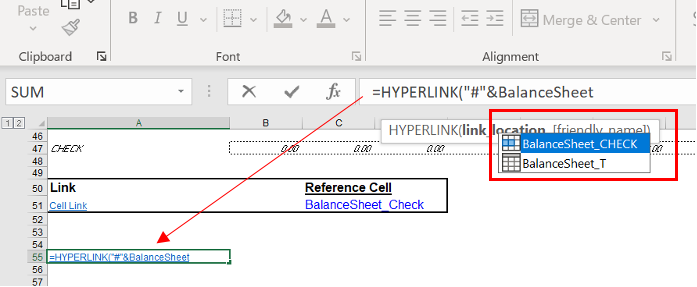
Excel will also provide a list of existing defined names that match what you start to type if you start typing the name of the cell after entering “#”& without the double quotation marks. Once your desired name is selected, add the double quotations around it. This ensures that the function works properly.

Hyperlinks are extremely valuable tools to create an easy navigation system for model users. With the techniques noted above you can avoid common problems. Make sure that your models remain organized and easy to use.