
Dynamic Arrays Part I – The Biggest Change to Excel in Years
Over the years, changes to Excel’s software tend to be slow, incremental, and nearly always backward compatible. One of the requirements of maintaining software in use by hundreds of millions of people worldwide. However, the latest Excel versions have introduced a feature that changes the fundamental way spreadsheets can be used, Dynamic Arrays.
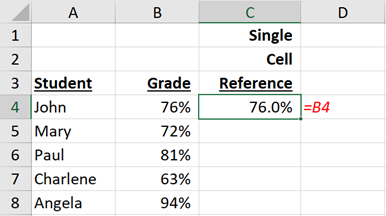
In the past, you would enter a single formula into a cell and it would return a single result. If you want additional results, you would need to copy the formula down. For example:
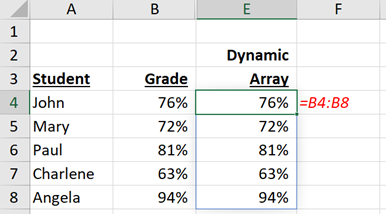
Dynamic Arrays add an entirely new way to use spreadsheets. It’s now possible to enter a single formula that returns a range of results across several cells (as seen below).
Avid users of Excel will notice that this is similar to previous Array behavior in Excel. For example, in formulas, you would enter a range of cells by entering CTRL + SHIFT + ENTER. Dynamic Arrays dramatically simplify and expand the use of this behavior and avoid many of the shortcomings of the classic Array feature in Excel.
Key to understanding this new feature is to realize that you are only entering the formula in one cell (in the example above, in cell E4). The results of the formula “spill” out of the cell to create the Dynamic Array. The cells below E4 (for example, cell E5), contain information but do not have an actual formula. Selecting the cell will grey out the text in the formula bar. This indicates that the cell contains results “spilled” from a formula in a different location.
![]()
At first, these formulas look like an alternative to copying across a range. But Microsoft has also introduced many new functions that take advantage of this behavior. There are a few older functions that can leverage this functionality as well. A key to using these new features is to understand that the size of the resulting Dynamic Array can change automatically depending on the values that you provide to the formula.
New Excel Functions Using Dynamic Arrays
- UNIQUE: Returns a Dynamic Array with a list of unique values in a list or range. Previously this was a common task that was much more difficult with “standard” Excel functions.
- FILTER: Create a Dynamic Array filtered based on criteria that can be changed.
- SORT: Sorts the contents of a range with the ability to specify which column to sort by ascending/descending order
- SORTBY: Sort the contents of a range with the ability to sort based on multiple columns in either ascending or descending order.
- SEQUENCE: Create a Dynamic Array with a sequential list of numbers with the ability to set starting value and the “step” for each sequence.
- RANDARRAY: Create a Dynamic Array with a list of random numbers (either integers or decimal numbers)
Dynamic Arrays with the OFFSET Function
One of the most valuable uses of Dynamic Arrays is to create lists that update automatically in conjunction with the OFFSET function in Excel. Excel’s offset function will start from a reference cell, move a certain number of rows or columns in any direction, and return the value in that cell.
OFFSET also has two additional arguments that allow you to return an array of values of a certain width or height. Before Dynamic Arrays, these OFFSET functions would be used with Dynamic Named Ranges (a topic for another day and covered in Marquee’s Excel 2: Advanced Data Analysis course) or with Excel’s previous Array behavior (CTRL + SHIFT + ENTER). With Dynamic Arrays, much of OFFSET’s power has been unlocked with the ability to display extremely customized lists from large datasets. In the example below, we use an OFFSET formula that will allow us to display the first X values in the list (7 in our example). This can be changed on the fly and the list will automatically update.
BUT WAIT! I like the new functions, but I want OFFSET functions in Excel to work like they did back in 2003! Never fear, see the endnote at the bottom of this article to learn how to do that.
Potential Dynamic Array Pitfalls
Dynamic Arrays are very helpful and create new and powerful ways to use Microsoft Excel. It’s important to understand any limitations before putting this functionality “into the wild” in your spreadsheets.
-
SPILL errors:
- The behavior change where a single formula may return results across a range of cells introduces some new issues. You may find that Excel is unable to return the range of information that you have requested. This will generate a #SPILL! error. Reasons that you may get a spill error include:
– The spill range has other information in it already
– Excel can’t determine the size of the array being spilled because it is volatile (i.e. using a random number to define the size of the Dynamic Array
– The result extends beyond the boundaries of the workbook
– The formula is in a Table (Dynamic Arrays formulas will not work inside a Table, but Dynamic Array formulas can refer to a Table)
– The result is too large and Excel has run out of memory
– The result is spilling into a merged cell (another reason to avoid the use of merged cells in spreadsheets)
- The behavior change where a single formula may return results across a range of cells introduces some new issues. You may find that Excel is unable to return the range of information that you have requested. This will generate a #SPILL! error. Reasons that you may get a spill error include:
-
Backward compatibility:
- Dynamic Arrays are only available on Microsoft 365 versions of Excel (Current Channel). It’s not available on Excel 2019/2016 (or earlier versions). If you save a worksheet with Dynamic Arrays and somebody tries to use the sheet on an older version of Excel, the Dynamic Arrays will be converted to traditional Arrays. This can cause a loss of functionality or unexpected behavior.
-
Creating unnecessary complications:
- Training The Street always believes you should use the simplest, most understandable features in Excel to accomplish what you want. While Dynamic Arrays add interesting new ways to analyze data, you should give some thought to whether Dynamic Arrays are the simplest approach possible.
Dynamic Arrays are an exciting new feature in Excel; we look forward to seeing new and creative implementations of these functions in financial modeling & analysis as they become available to more Excel users!
——
ENDNOTE:
New things frighten me. Sometimes we just want things to work like they did back in Excel 2003. When the paste special shortcut was Alt -> E -> S -> F, when 50 Cent topped the charts, and when popped collars were finally making their comeback.
We can force Excel to stop spilling and return a single value from the resulting array by using the @ symbol after the equals sign (i.e. =@OFFSET(B3,0,0,H2)). This is called the intersection operator and will return a single result from the array that is on the same row (or column) that the formula is entered in.
The intersection operator (and its cousin, the spilled range operator (#)) allow for some interesting other behavior with Dynamic Arrays. However, this article is long enough as is; we will return to this topic before long.
Training The Street also offers a more advanced In-Person/Virtual Public Course called, Applied Excel. Where you can gain the skills needed for parsing, analyzing, and presenting information from large data sets.