
Custom Number Formatting in Excel
Part 1
Almost every Excel user has faced the need to format data in their spreadsheets in some way, shape, or form. Not surprisingly, this task can often lead to multiple trips to the formatting ribbon. Wouldn’t it be nice to be able to format data in one simple step so that it is displayed as per your specific requirements? Come to the rescue Custom Number Formatting!
At TTS, we are strong advocates of presenting data in a clear, logical, and user-friendly manner. Custom Number Formatting allows a user to format the contents of a cell in a multitude of ways. The focus of this article will be on the basic syntax that is followed and to provide a simple example. Another fundamental principle at TTS is Excel efficiency which typically translates to minimal use of the mouse. As such, certain Excel keyboard shortcuts will also be mentioned throughout the article to enhance user efficiency.
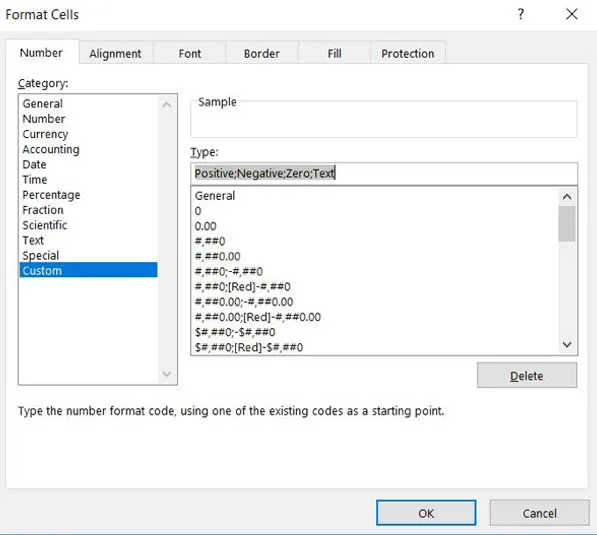
Many people know that to format a cell, they can right-click their mouse, click on Format Cells to open the Format Cells Dialogue Box, and then apply the necessary formatting. However, what many people do not know is that the same box can be opened by simply hitting CTRL + 1. Once open, you can apply a custom number format by hitting the “Tab” key to get to the Category list and then by pressing the “C” key twice to get to the Custom field (it will be highlighted if done correctly). Now press the “Tab” key to get to the Type box – this is where you can define a custom number format in the following sequential syntax order: Positive;Negative;Zero;Text. Colour can also be added to the format by putting [color] before any of the above inputs. The diagram below shows a visual depiction of the Format Cells Dialogue Box and the syntax described above.
Example:
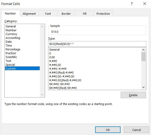
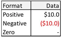
Let’s look at an example where the model/user requirement is to have positive numbers to one decimal place displayed with the $ sign, negative numbers to one decimal place displayed with the added formatting of parenthesis and red font, and a zero to be displayed as “-“.
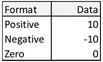
To demonstrate, we will use the data set below as our sample (Assume the data is in cells B3:B5).
To convert the above data to our desired format, please follow the steps below:
Step 1: Highlight the Cells to be formatted (e.g. cells B3:B5)
Step 2: Hit CTRL + 1 to open the Format Cells Dialogue Box and navigate to the Custom Number Type box (see above)
Step 3: Type $0.0;[Red]($0.0); “-“;
Note: This is the format required in this specific example. It is here where there are numerous options and formats for users to define.
Step 4: Press ENTER and Voila!
Part 2
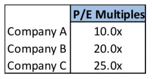
We can now expand on Part 1, by demonstrating how to combine letters and numbers in a cell. Consider a situation where we would like to show the P/E multiple for Companies A, B, and C in the table below. These values would then be used within calculations in different parts of a spreadsheet.
If we just typed “10.0x” into the cell for Company A, the value would be transparent and intuitive but not dynamic or flexible because it could not be used as an input for any calculations. Why? Because Excel would recognize the cell as text due to the “x” being directly in the cell.
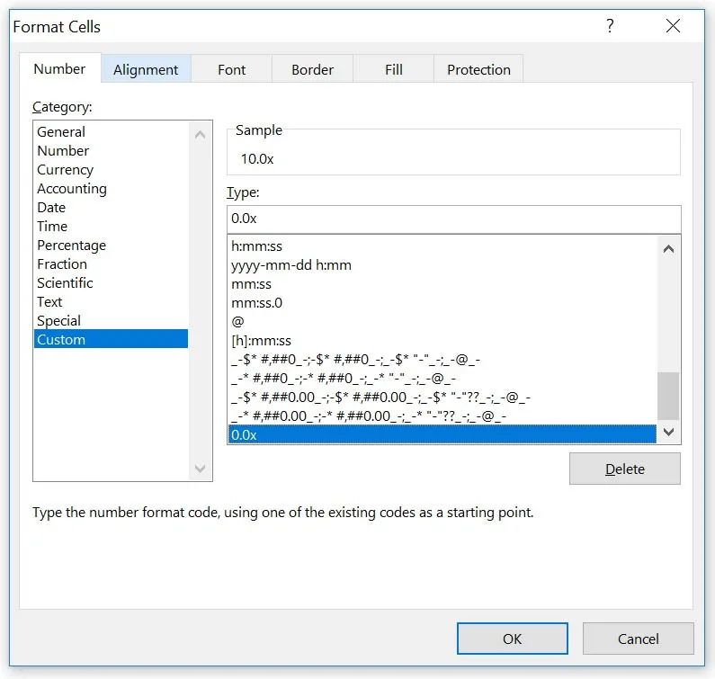
Custom Number Formatting to the rescue! In the format dialogue box below (hit CTRL 1), select the Number tab, choose Custom, and then navigate to the section labeled “Type”. We can now define our Custom Number Format as 0.0x. Zeroes act as placeholders for each digit in the number to be displayed. Since we want our number to end with an “x”, which is a text character, we place the x after the zero placeholder. We don’t need quotes around the x which is often the case for single letters in other custom formats.
We are now able to enter the number 10 into the cell but it will be displayed as 10.0x. By using Custom Number Formatting, we have ensured that the multiple can be used in calculations throughout the spreadsheet.
If these were inputs for a working capital schedule, then we may want the inputs to read as “10.0 days”. We can again use Custom Number Formatting and enter 0.0 “days” in the custom formatting box. Note that double quotations are needed when there is more than one text character.
This is just one of the many ways you can use Custom Number Formatting in your Excel files.
Training The Street also offers a more advanced In-Person/Virtual Public Course called, Applied Excel. Where you can gain the skills needed for parsing, analyzing, and presenting information from large data sets.