Help, I Am Lost in this Massive Excel File! A Short Guide to Hyperlinks in Excel

Have you ever opened an Excel file and seen multiple tabs each containing multiple schedules? Did you start working through the file and find yourself frustrated going back and forth between different schedules and / or tabs? In this article we will address these issues and provide some helpful ways to navigate through a long complex file in a seamless manner. Specifically, we will show you: (i) how to insert hyperlinks (ii) some tips and tricks to make hyperlinks more user friendly and (iii) a sample table of contents we build into many of our consulting models.

Benefits of Using Hyperlinks

The primary benefit of using hyperlinks in an Excel file is to allow a user, through the simple click of a mouse, to navigate between different locations within a file. Hyperlinks also serve as a communication tool since the text displayed as a hyperlink provides a description to the area where a user will be navigating to.

How to Insert Hyperlinks

Step 1: Locate the cell where you would like the hyperlink to appear.

Step 2: Once the cell is selected, open the hyperlink dialogue box using the keyboard (Ctrl + K).

Steps 3-7 all occur within the dialogue box (see figure below).

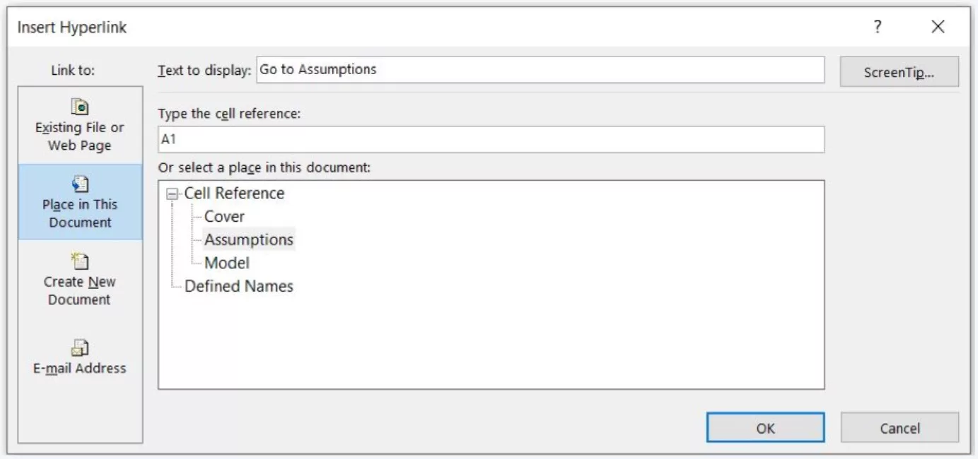
Step 3: On the left-hand side under the “Link to” area, click on “Place in this document”.

Step 4: In the “Text to display:” section, type in the text you would like to display in the cell. In the example below we would like to display “Go to Assumptions”.

Step 5: In the “Type the cell reference” section, type the cell reference you would like to be navigated to after clicking the hyperlink. Note: Excel defaults to cell A1. We have kept it at the default A1 in the example below.

Step 6: In the “Select a place in this document” section, choose the location (i.e. tab) where you would like to be navigated to after clicking the hyperlink. Note: Excel defaults to the current tab if you do not choose a specific tab for the cell reference. In our example, we have three tabs in our Excel file and have chosen the Assumptions tab.

Following the above steps, a similar dialogue box to the one below should appear on your screen.

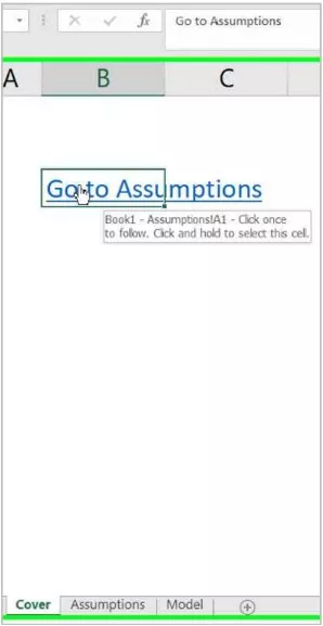
Once you click OK, the hyperlink will appear in the selected cell and if you hover over the cell you should see the cursor change from a “plus” sign to a hand sign (see below). In our example, clicking this cell takes you to Cell A1 on the Assumptions tab.

Making Hyperlinks User-friendly

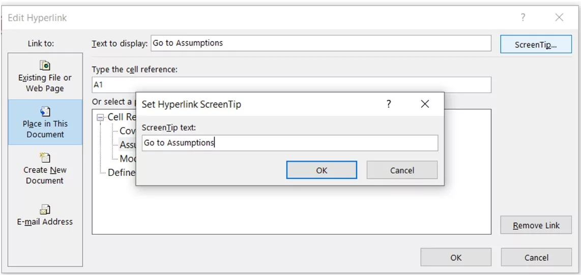
The first thing you might notice in the figure above is the text “Book1-Assumptions!A1…” that appears when you hover over the hyperlink. Excel is providing the location of where the hyperlink will be taking you. At Marquee, one of our guiding principles is to make financial models as user-friendly and aesthetically pleasing as possible. Wouldn’t it be nice to be able to change the wording of this text to something more intuitive like “Go to Assumptions”? To do this you would need to navigate back to our dialogue box (Ctrl + K) and click on the Screen Tip button. In the Screen tip dialogue box you can then type in the text you want to appear (see below). Press OK. Now, when you hover over the hyperlink you will have resolved the above issue.

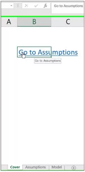
As you can see, when you hover over the hyperlink the text that appears is much more relevant to the contents of the model.

Marquee and Hyperlinks in Practice

Did you know Marquee has a robust and growing consulting practice, where we work with a wide array of clients to build dynamic financial models and/or custom data solutions? The models we build often have numerous tabs and many individual schedules on each tab. We always include a Table of Contents tab (see below) with hyperlinks to make navigation as easy as possible for our clients. In the General section of the figure below, each one of the boxes is a hyperlink to its respective tab within the model. This serves two purposes: the hyperlinks not only help a user to navigate the model but are also a great communication tool.

To associate a hyperlink to a shape (as in the figure below), we must first insert a shape (Insert > Shape). Click and draw the desired shape (the cursor should change from a thick plus sign to a skinny plus sign) and then follow the steps above to associate the hyperlink to the shape. Remember when creating a hyperlinked shape that you must type your desired text directly into the shape, not the dialogue box (see Step 4 above).