On Your Marks, Get Set… Using Excel’s SUMPRODUCT Function
This article is for all the teachers out there. We love teaching at Marquee and in addition to our numerous training programs we also teach some University courses at business schools. So we know that March is often “Marking Month” after all the mid-term exams that occur before reading week. In this article, we want to share a cool little formula to help ease that crush, improve accuracy, and make the marking process a little easier. If you don’t have exams to mark, it is still a helpful feature of Excel that has many other applications.
The Situation
Let’s start by showing the test results and the answer key for the exam that we need to grade. It’s a multiple choice test with possible answers of A through D.
Figure 1
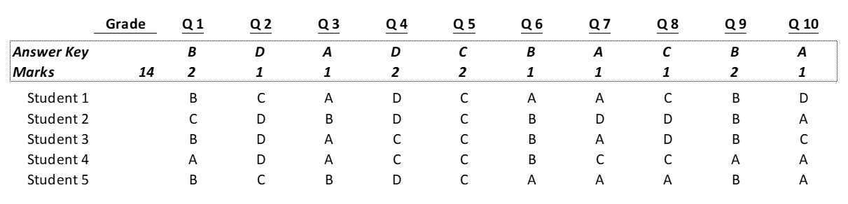
Students will receive marks for each correct answer. In Figure 1, Student 1 got Question 1 correct and receives 2 marks for that answer. They answered Question 2 incorrectly (they entered C not D) and therefore receives zero marks. The test has 10 questions that add up to 14 total marks.
Entering Things Properly
For this quiz, how do we ensure that we only enter an A, B, C or D in the response fields?
This restriction is easily done with Data Validation. Once data validation is completed for a single cell it can be copied throughout the area for student answers. The figure below shows the menu for the validation that will allow us to restrict inputs to the four letters that we need. These have been entered in cells off to the left of the data input. The Data Validation menu can be found under Data>Data Validation>Data Validation. We select “List” in the Allow field, and highlight the cells holding the letters in the Source field
Figure 2
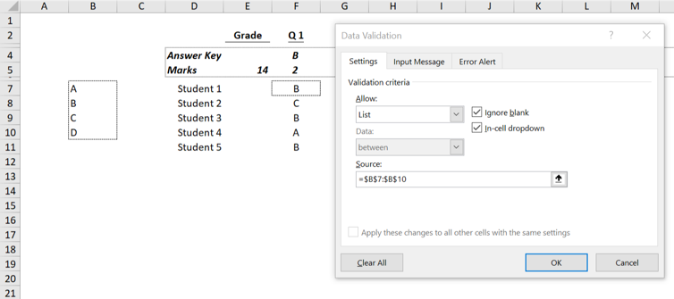
The Data Validation instructions in Figure 2 will restrict the contents of the selected cell (in this case F7) to only the list of inputs contained in cells B7 to B10. Now we can’t sneak in an “E” by accident.
Getting the Results
Once the answers have been entered into our grading spreadsheet, we still need to check each answer against the answer key and then assign the correct amount of marks to each response. Last, we will need to total those individual marks to arrive at the overall grade.
One way to do this is use one IF function for each response. We would build a second table of IFs below or beside the results table and then add up each row for each student. The IF function would look like this:
=IF(Student Answer = Answer Key, Marks for Question,0)
This means that we have to repeat the table again and make sure everything is linking properly. It’s doable but it would be nice to perform all these calculations in one spot and simplify our spreadsheet.
SUMPRODUCT to the Rescue
SUMPRODUCT is one of the most flexible and powerful functions in Excel and it has more uses than many users realize. It allows users to work with arrays of numbers not just individual cells. There is a class of functions in Excel called Array Functions that also work with arrays (you can spot them because the have {} brackets around them) but these functions can be inflexible and complicated. Built properly, SUMPRODUCT can give you the same power without the complexity of Array Functions.
SUMPRODUCT’s basic ability is to multiply arrays of numbers and then add them up. In figure 3, we have two arrays that we wish to multiply together. The answer should be 30.
Figure 3
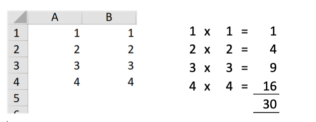
This operation can be done using SUMPRODUCT as follows:
=SUMPRODUCT(A1:A4,B1:B4)=30
We can already see that this will be useful in calculating each student’s score (marks per question x number of questions correct) but we still need a way to determine if the student answered each question correctly.
Previously we used IF functions to do this but now we will use another feature of SUMPRODUCT to build our final formula.
SUMPRODUCT as a Search Function
The SUMPRODUCT function can multiply arrays as we have seen above but it can also perform logical tests on arrays as well. Using the example below we can find out which rows have the same numbers in both the red and blue boxes. The formula we will build to do this uses an equal sign between the arrays instead of a comma.
Figure 4
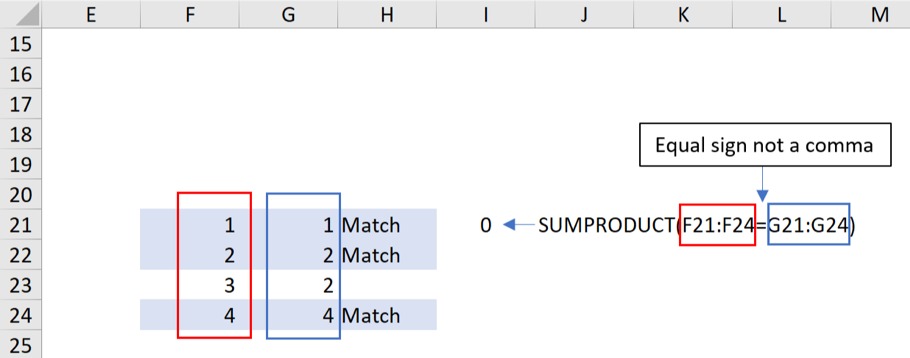
You will notice the output of this formula is currently a zero! It should be “3” since there are three rows (highlighted in blue) that match and therefore should give a TRUE value. Why does this appear not to work? In Excel, TRUE can often be replaced with a 1 and False a 0. But If we look at what the formula is adding up would we see the following:
SUMPRODUCT({TRUE;TRUE;FALSE;TRUE})
We need another function to convert these values from TRUE/FALSE to numbers. The N() function is designed to do exactly this. Our updated formula that will give us a “3” for the three matching rows is:
SUMPRODUCT(N(F21:F24=G21:G24))
You may have seen other model builders multiply the formula by 1 to achieve the same result:
=SUMPRODUCT(((F21:F24)=(G21:G24))*1)
Putting it All Together
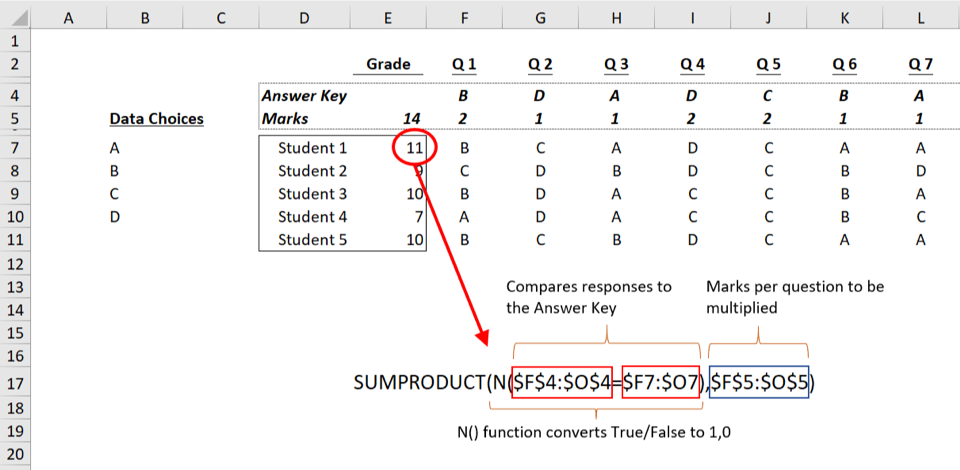
Now we are ready to combine all the features described above to create one formula that will to calculate each student’s result on the test:
- Figure out which questions were answered correctly
- Multiply by the points awarded for each question
- Add it all up for the final mark
Figure 5 shows the formula below the table that is used in the grade column next to each student. Any time you need to match and multiply, SUMPRODUCT is the tool to consider.
Figure 5