
Excel Hacks – My Favourite Spreadsheet Speed Tips and Tricks
Necessity is the mother of invention. Something’s not working and we have to figure it out. It applies to all sorts of things in life.
Late at night, we are battling a pesky error message and after some Google searches, we find a workable answer. It’s not very elegant – it works but it’s not great. Of course, by this point, it’s always late and we move on hoping to never encounter the error again.
Sometimes it’s not even an error – we find we are always repeating actions in Excel that require several steps that feel redundant. Saving time requires research – spending time to save time can be hard to budget. Using the ALT key and the keyboard commands is always recommended but there are a bunch more. This article series is meant to do just that and share some of my favorite Excel hacks. This article provides two of my simple favorites:
- Quickly check a range that Excel automatically selects; and
- Fixing all my formulas at once
Quickly Checking a Range
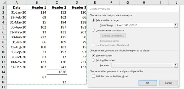
Lots of tools in Excel will automatically “grab” a block of data to be used by that tool. An example is Pivot Tables that will automatically select any block of data near the cursor. Ideally it grabs all the data you want and the headers for the data. But if there are some formulas and calculations underneath or beside the data, Excel may grab too many cells and include blanks and other cells that should not be selected. As I like to say, I may love Excel but I don’t trust it – you should always double check what Excel selects.
This example shows what can happen – too many rows in the range. We can delete the range selected and redo it but you can save time with a little trick – Hit Shift and use your up and down arrows to move the bottom of the selected range. If the range is good then move the selection range back to where you started. But in the case below, we would move the arrow up three rows to exclude the “junk” underneath the data. Just hit Tab to navigate away from your corrected Table/Range.
Fixing All My Formulas at Once
This is a great tip especially if you are prone to do what I often do – fix the first formula in a schedule and then keep fixing other formulas in the same column. If I move on I will have forgotten to copy the fixed version across the rows and now I have a mix of fixed and erroneous formulas. To avoid this I use this Excel hack and changed my process when fixing formulas:
- Select the first formula to fix and then CTRL + SHIFT + Right Arrow to highlight the entire row
- Hit F2 (CMD + U if you have a Mac) and fix the first formula
- Final step – THIS IS THE KEY! – CTRL + Enter.
You have now copied the fixed formula instantly into the entire row in one step and it won’t affect your formatting!
If you enjoyed reading this and want to improve your skills further, then try our Excel Best Practices Self-Study Course. You can also browse our other range of Self-Study Courses here.
Training The Street also offers a more advanced In-Person/Virtual Public Course called, Applied Excel. Where you can gain the skills needed for parsing, analyzing, and presenting information from large data sets.