
Top 5 Time-Saving Tips to Automate Excel Charts
Data analysis, communication, and visualization continue to grow in importance and popularity. At TTS, Data Analysis and Communications with Excel, Power BI, and Python Training (Part 1 and Part 2) are among our fastest-growing, highest-demand courses, so it’s important to learn and utilize time-saving tricks to help you with automating your Excel charts.
While Power BI and Python are powerful data representation tools, the majority of professionals continue to chart their data in Excel (assuming their data sets have not outgrown Excel’s capabilities). We have spent countless late nights tediously creating and updating charts in Excel, which is why we especially want to share these immediately-applicable, time-saving tips to automate your charts:
1. Reference a Dynamic Data Source
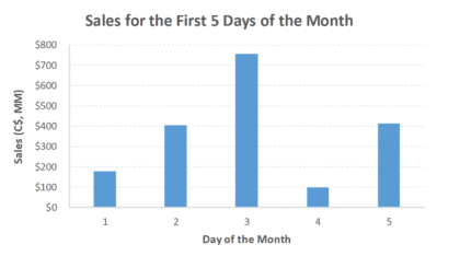
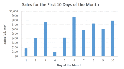
If you expect your data set to grow, we recommend referencing a dynamic data source for your chart. For example, the chart on the left was created using all available sales data on the 5th day of the month. The chart on the right was created using all available data on the 10th
If the first chart was created by sourcing a static range (i.e. A2:A6), then on day 10 you would have to tediously update your chart manually by selecting an updated static range (i.e. A2:A10). However, if you originally created the first chart by sourcing a dynamic range (for example, you can create and reference a Table or a Dynamic Named Range), then, on day 10, your chart will automatically be updated.
2. Ensure All Text is Dynamic
We want all aspects of our charts to update automatically, including any text in the chart (such as data labels, sub-titles, and titles). In our example above, we want to ensure the title automatically updates along with our data when we update the chart on day 10. In order to do so, we used Excel’s Concatenate Function to make the title dynamic.
3. Link Titles to Dynamic Text
Next, we link the chart title to the dynamic text to automatically update the chart title. In this case, we selected (left-clicked) the chart title, hit “=” (you will notice an “=” sign in the formula bar), and linked to cell D1 (which contains our concatenate function). The same technique can be applied to axis titles and sub-titles.
4. Link Text Boxes to Dynamic Text Too
Text boxes can also be linked to cells in Excel.
However, when you click on the text box, you must type “=” directly into the formula bar. Typing “=” after clicking on the text box will treat the “=” as text within the text box. In addition, you can also type F2 to access the formula bar.
When inserting a text box into a chart, grouping the text box with the chart is also helpful. You can do this by selecting the chart before inserting the text box. Another way is by highlighting the chart and text box > right-click> Group). If the two are ungrouped, the text box will not move when the chart is moved.
5. Paste as a Linked Picture
If you need to paste a copy of your chart to another area of your worksheet or workbook, it’s not ideal to paste it as a picture because a picture is not “live”. It will not update when you change your original chart. Instead, copy and paste your chart as a Linked Picture. You can do this by selecting all the cells behind your chart > CTRL + C > Home > Paste > Linked Picture. Note the Linked Picture is “live” with a view of the cells you highlighted before copying. It will therefore update as you change your chart. You may want to turn off gridlines (View > Gridlines) so they don’t appear in your Linked Picture.
If you enjoyed reading this and want to improve your skills further, then try our Excel Best Practices Self-Study Course. You can also browse our other range of Self-Study Courses here.
Training The Street also offers a more advanced In-Person/Virtual Public Course called, Applied Excel. Where you can gain the skills needed for parsing, analyzing, and presenting information from large data sets.