How to Use the INDIRECT Function in Excel

Many people have either seen the INDIRECT functions in spreadsheets or heard of it. Most, however, don’t understand its purpose. INDIRECT can be extremely useful in certain situations.

In a nutshell, INDIRECT allows you to connect strings of text to look like a formulaic cell reference, and have Excel treat the result as an actual formula. This is useful especially when you need a summary sheet to pull data from various other sheets or files. Normally setting up a summary sheet involves a lot of tedious, manual linking. But when the data is laid out in an organized way on various sheets, INDIRECT can help us create a dynamic formula that can be copied and pasted instead of having to link multiple times.

When you link a cell to a cell on another sheet, the result looks like this:

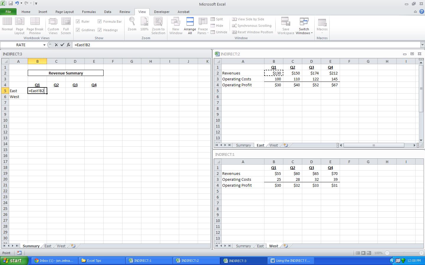
Notice that the cell reference has the following components after the = sign:

1. The destination sheet name (East)
2. An exclamation mark (!)
3. The destination cell reference (B2)

Once the Q1 revenues are linked in the example above, the manual way to proceed would be to continue to link cells one by one. This is where INDIRECT comes into play.

Take a look at the revised version below:

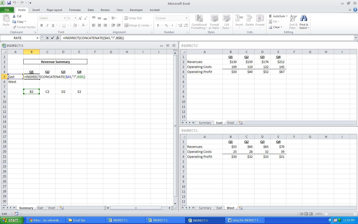
Recall that the CONCATENANTE function (or the & sign) allows you to connect, or join together, strings of text, even if these strings are in other cells. On its own, the result of concatenating various components will be a string of text. In the formula above, we concatenated the sheet name, the exclamation mark and the cell reference (i.e. to create the text string “East!B2”). By putting this inside the INDIRECT function, however, we tell Excel to treat the result as a formulaic cell reference. Since the data for Q1-Q4 are organized in an identical way on both the East and West sheets, we manually typed the cell locations below the summary table. With the appropriate absolute references, the formula can be copied to fill in the whole table.