The Quagmire Challenge: Guest Lists (September 2017)
The Question
In this Challenge, you will have to use a few different Excel techniques. Consider the following situation: your company has decided that it wants to host a lunch & learn with the new CEO. As the Excel guru, HR has asked for your help with this task. They have provided you with the full names of the company’s 300 employees. Unfortunately, due to a glitch in the HR system, all the names appear in a random order.
If you click here you can download the spreadsheet with the sample data.
There are enough seats in the Executive lounge that up to 40 employees can have lunch with the CEO per session. The sessions will be grouped by the first letter of the attendee’s last name. Twenty-six separate sessions have been booked with the CEO, one for each letter of the alphabet. The department wants to keep track of invitations alphabetically and needs a way to select names from an alphabetical list one at a time.
As the efficient Excel user that you are, you know that you can save time by building a tool to generate a guest list with the following requirements:
- A drop-down list of names (grouped by last name in alphabetical order) based only on the selected letter of the alphabet (i.e. all employees whose last name starts with A, all employees whose last name starts with B, etc.) from which names can be selected for emails
- No macros
- No VBA
Your solution might look something like this:
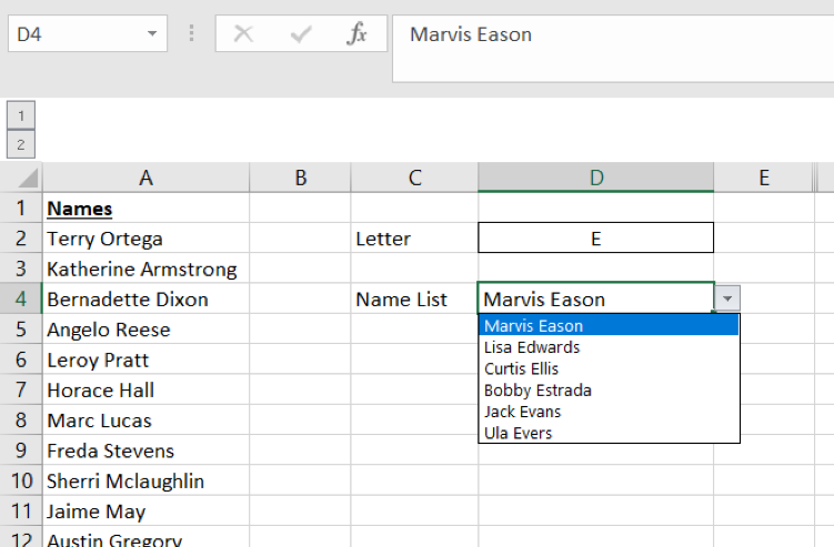
To make life a little easier, we have included a drop-down list of the alphabet in the spreadsheet. We have also included headers to give you a few ideas.
The Solution
As with all of our Quagmire challenges, there are multiple ways to handle the problem. In the solution below we highlight just one approach.
- Find first letter of last name
It’s possible to use any number of combinations of text functions to extract the first letter of the last name, but we prefer this simple one (assuming the name is in cell B9):
MID(B9,FIND(” “,B9)+1,1)
- Create a filtered list of names that have the selected letter as the first letter of the last name
In order to create a filtered list, it is necessary to identify the location (“Row Number”) of matching criteria in the data set (“Name List”). This can be done in either two steps or one.
The first of two steps is to put the row number next to only those names which match our criteria. When the criteria letter is in cell D2 and the list of first letters is in column H, we can use the following formula:
IF(H21=$D$2,COUNTA(H$2:H21),””)
Take note, the COUNTA() has an expanding range.
The second step is to consolidate this list using the SMALL() function.
To complete this in a single step, you can use a MATCH() function with a dynamic lookup array (using the OFFSET() function).
Once you have developed the applicable list of row numbers, you can create the list of filtered names using the INDEX() function:
INDEX(“Name List”, “Row Number”)
- Use text formulas to rearrange filtered names into “Last, First” format
Again, it’s possible to use any number of combinations to do this, but we prefer this simple one (assuming the filtered name is in cell J9):
MID(J9,FIND(” “,J9)+1,LEN(J9)-FIND(” “,J9))&”, “&LEFT(J9,FIND(” “,J9)-1)
- Find the rank of each filtered name within the set
Unfortunately, the RANK() formula does not work with text. Luckily, COUNTIF() does work (albeit, in a slightly more complicated way). Therefore, we can use the following formula:
COUNTIF($Q$3:$Q$42,”<=”&Q3)-COUNTIF($Q$3:Q3,Q3)+1
Take note, the second COUNTIF() has an expanding range. In the case of a tie, the names would appear in the same order as they do in the filtered list.
If you were certain all of your values were unique, you would only need a single COUNTIF() and could use “strictly less than” as your criteria.
- Arrange filtered names into alphabetical list
This can be done using a simple INDEX() / MATCH() combination or VLOOKUP().
- Create a drop down using the sorted filtered list
This can be done simply using Data Validation. To eliminate the extra spaces, you can use a Dynamic Named Range.