The Quagmire Challenge: Timing Trifecta (June 2017)
The Question
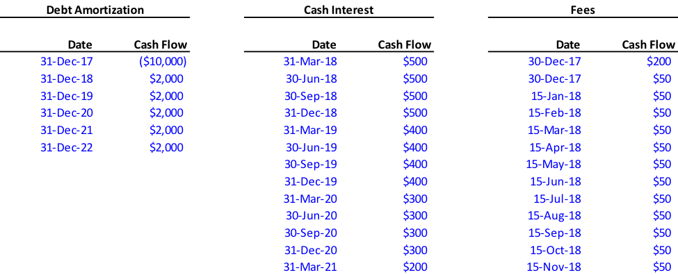
The XIRR function is relatively well known by most Excel power users. However, XIRR requires all the dates and cash flows to be in two distinct arrays. But what if the contemplated investment being analyzed contains multiple components each with different dates? For example, consider an investment that contains
- A 5-year debt instrument with annual year end amortization;
- Cash interest paid at the end of each quarter; and
- An initial fee plus a regular fee payable on the 15th of each month
If you click here you can download the spreadsheet with the sample data for the problem.
Using a series of dynamic formulas, create a unified set of cash flows and calculate the blended IRR.
The Solution
As with all prior Quagmire problems, this one can be solved multiple ways. Although it is technically possible to calculate the IRR for this set of cash flows using just a single formula, we prefer to create a single stream of cash flows as it provides additional insights into the data.
The solution can be thought to have four functioning parts:
1.Create a unique set of dates. The first step is to create a new section that contains all the dates to be considered. This section is comprised of links to the original raw data.

If there were no repeating dates, we could create a standard ranked table where the ranks are calculated by adding 1 to the previous rank (with the first number [1] being a hardcode). If we are populating a rank in cell U7, the formula would look like this:
=U6+1
As you can see in the data set above, there are a number of dates that appear more than once. As such, we will need to use a different formula to create the ranks. We prefer using the below COUNTIF formula as it is simple and easy to understand. In this example, we are populating the rank in row 7, and our data set of dates is in the range of Q5:S126.
=COUNTIF($Q$5:$S$126,”<=”&V6)+1
The corresponding ranked dates can be filled in using the SMALL formula (with the data set of dates as the “array” and the rank as “k”. The finished output will look like this, note how the rank skips from “1” to “3”, as there are two “30-Dec-17” in the data set.

2. Aggregate cash flows for each date. Now that we have the dates, we need to add the corresponding cash flows. This can be done a few different ways, but in this case we would prefer to use a series of SUMIF functions. The formula would be structured like this (in this case we are populating the cash flows for the date in cell L6):
=SUMIF([Date range #1],$L6,[Cash flows range #1])+ SUMIF([Date range #2],$L6,[Cash flows range #2)+ SUMIF([Date range #3],$L6,[Cash flows range #3)
There are more complex formulas that use the SUMPRODUCT function to achieve the same result, however, we prefer the SUMIF function here because it is better understood. You wouldn’t want to use an INDEX / MATCH function combination in this situation because there might be more than once cash flow for the same date (like the first two under “Fees”).
3. Use an IRR starter. The XIRR function won’t work unless the first value is a negative number. In this case, the first negative value wasn’t until the third date. Instead of rearranging your data, add a space before your data. Set the date equal to the date of your first cash flow and enter a very small negative value (i.e., -110-100) for the value. If the number is sufficiently small it won’t have any impact on your IRR.

If you don’t believe us, try it for yourself.
4. Check with Manual Method. The solution from above can be checked by copy (CTRL + C) and pasting (CTRL + V) the dates and cash flows into a single continuous array with one group below the previous one. The XIRR function can then be run on this set of dates and cash flows. Remember to use the IRR starter!