Getting a Unique List with Google Sheets
I talked in the last article about some of my favourite shortcuts and several of you responded with some of your own. Please keep them coming and, as a reminder, the best ones will get rewarded with a Das keyboard!
For this article I am taking a detour from shortcuts to talk about a common data problem that I run into and a surprisingly quick way to manage it. At Marquee, we have begun doing more training on Google Sheets. It is very similar to Excel (and you can select a button on the Google Sheets menu to use your Excel Shortcuts – hit CTRL / to open the menu) there are some interesting differences.
A common issue I have is figuring out how many unique records I have in a database and then figure out how many of each I might have. For our webinars we might have attendees from around the world and I often want to know how many people attended from a specific city. If I have 300 attendees for the webinar, what is an easy way to know the participants’ home cities.
Both Excel 365 and Google sheets have a function that will answer this question for me. In the sample below I have used a UNIQUE function to extract one example each from the list of cities in Column B. If I want to see that list in alphabetical order, I have wrapped the UNIQUE function with a SORT function and declared the third argument (the is_ascending argument) to be True so that the list is alphabetical.
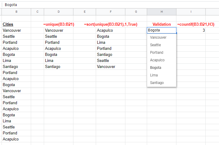
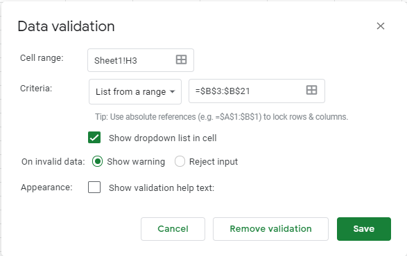
You will also notice a label called validation. I have created a drop down list in cell H3 using Data Validation, which I created using the menu below found in Data > Data validation. Here is a unique advantage of the Data Validation feature in Google Sheets – it automatically creates a list of unique entries when you highlight your data set! There is no need for the UNIQUE function. With this list I can now drive another function easily such as the COUNTIF function to determine the number of attendees by city. In Excel I would have had to build the drop down list from the output of the UNIQUE function.