Terminal Value – Perpetuity vs. Multiple Approach
How to Determine the Intrinsic Value of a Stock
To determine the Intrinsic Value (IV) of a stock, investors need to try to determine the present value of a company’s future cash flows that are attributable to equity investors from now until… INFINITY. Today, we are going to take an in-depth look into two approaches that help simplify this process for investors.
First, let’s unpack the formula for determining the IV of a stock:
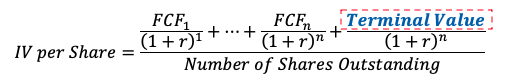
There are two parts to calculating IV, the first part is to determine the value of future cash flows that need to be forecasted on a year-over-year basis. The art of forecasting future cash flows on a year-over-year basis is something we cover extensively in our Building a Financial Model course.
The second part, Terminal Value (TV), is what we’ll spend our time understanding in this note.
Why Terminal Value is Crucial to Valuation
Even the most talented investors are limited in their ability to forecast more than a few years of Free Cash Flow (FCF) in a detailed manner. Typically, most financial models only incorporate 5-10 years of detailed forecasted FCF. So, if only 5-10 years of FCF is forecasted in stage 1, how does an investor determine the value of FCF in the 11th year? The 30th year? The 100th year? To answer this, we need to take a deep dive into Terminal Value.
The best, or most correct, way to calculate terminal value is the ONLY time in finance where Academics and Practitioners disagree (if only this were true)! If you went to business school, chances are your Finance Professor walked you through the first method of calculating Terminal Value: The Perpetuity Approach.
- The Perpetuity Method
Understanding the Concept of Perpetuity
This approach consists of trying to mathematically compute FCF from the final forecast year, until… infinity! As usual the Academics want to work with a concept that’s as confusing as infinite time! Professor Dunbar, I’m completely joking – everything you said about the Perpetuity approach does make sense from a theoretical perspective. Let’s take a deep dive into how investors can use the Perpetuity Approach to calculate Terminal Value.
First, we must understand the perpetuity formula. This is a simple formula that academics adjust to apply it to a stock’s valuation. The basic formula follows the following structure:
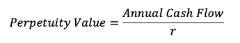
An example of when we use this formula in finance is to determine how much money someone needs in their retirement portfolio before they can retire. E.g., If you want to live on $50,000 of Pre-tax cash flow each year forever, and you can comfortably earn a 4% dividend on invested money, you need $1,250,000 invested. How this works conceptually is as follows:
- Your invested money ($1.25m) pays a 4% dividend = $50,000
- Withdraw the $50,000 from your investment account, you will still have the $1.25m left in your account to pay you the 4% dividend next year, and for the rest of time!
Computing TV Using the Perpetuity Method
So, how have Finance Professors and Researchers adapted this formula to estimate the IV of a stock into perpetuity? Let’s look at that below:
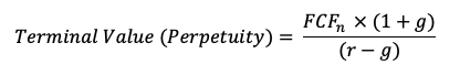
While there are different finance professionals and professors who will adjust this formula slightly, this is the formula in its most basic form. We take an annual cash flow attributable to equity holders that we expect to be indicative of normal business operations and free from cyclicality, then we manipulate it based on two factors: expected growth in free cash flow (g) and the Cost of Equity (r).
Understanding Cost of Equity
Cost of Equity, in simple terms, is the cost to the company for raising capital in the form of equity. To gain a detailed understanding of Cost of Equity as a concept and to see how it’s calculated in practice, please view our Valuation 1: DCF and Capital Structure Modeling Courses.
Understanding Terminal Value Growth Rates
The expected growth rate to use for the FCF is where this method of computing Terminal Value gets very interesting. Here, we must choose a growth rate at which we will value the stock into INFINITY which is surprisingly difficult to do.
If we use a growth rate for the stock that’s above the country’s GDP growth, that means we are effectively saying that one day this stock will become more valuable than the country itself. This is a big and risky assumption to make for a small growing company. But if we use a lower growth rate, we are also under appreciating the growth in FCF the stock may incur in the short-to-medium term after the initial forecasting period.
Because of the uncertainties and challenges associated with using the Perpetuity method, many practitioners find themselves using the second method of calculating Terminal Value: The Exit Multiple Method.
- Exit Multiple Method:
Understanding the Theory Behind the Exit Multiple Method
This method of computing Terminal Value is much simpler from an algebraic perspective. The logic used here is to determine how much the company could sell itself for at the end of the initial forecast period, and this value is equivalent to the pre-discounted terminal value.
The formula is as follows:
![]()
Picking a Financial Metric
The financial metric used will depend on the stock that is being valued. The investor will need to pick a financial metric that is usually a positive number for this industry’s incumbents (e.g., Revenue, EBITDA, etc.). For example, early-stage tech companies are often not very profitable, so the only financial metric practitioners have available to value them is their Revenue. If we compare this to the opposite side of the spectrum and look at strong stable cash flowing companies, they’re often very profitable, so practitioners prefer to use the EBITDA metric to value them as it’s the closest proxy for FCF that’s readily available or easily calculated.
Computing the Metric Multiple
The metric multiple used is related to the financial metric chosen. The value of the metric multiple used depends on judgment. Often, the median multiple across industry incumbents is used as a baseline for estimating value. You may use a value above or below the median if other analyses you’ve done suggests that the stock might be more or less valuable than its peers.
Important Thing to Consider Regarding Financial Metric Choice
An important thing to note is that most metrics will result in a computation of Enterprise Value (Value of the company) rather than Intrinsic Value (Value attributable to the equity holders). In these cases, we will need to deduct debt and any other debt equivalents and add back any cash and cash equivalents to equate the Enterprise Value to Intrinsic Value. This is an important step needed to compute the IV per share / what we believe to be the fair value of the stock price.
Metrics that will provide an approximation of Enterprise Value:
1. Revenue, EBIT, EBITDA, etc.
Metrics that will provide an approximation of Intrinsic Value:
2. Net Income, Dividends per share
Which Method is Best?
A. Pros of the Perpetuity Method
An advantage of using the Perpetuity Method is that this method is consistent with valuation theory. When a practitioner attempts to use the multiple method to determine the value of a company/stock in the event of a sale, they are using a simplified trading comp, which only approximates the Enterprise Value / Equity Value as judged by others in the market.
B. Cons of the Perpetuity Method
A disadvantage of using the Perpetuity Method is that it is not well suited for all companies. A new company with rapidly growing cash flows in the initial 5-year forecast period likely won’t see their growth in FCF drop below 4% in the short-medium term and their cost of equity will likely shrink as the stock’s risk profile lowers. But this won’t be captured under the Perpetuity Method as well as it can be captured by the Exit Multiple Method.
Another disadvantage is that this method can only be used for stocks expected to operate in a steady state forever. This is not a suitable assumption to make for many stocks (e.g., companies selling non-renewable resources, companies going through heavy restructuring, etc.)
C. Pros of the Multiple Method
A pro of this method is that it’s easy to understand and observable in the market. If the company was to sell itself, this FCF generated from the sale would be distributed to stakeholders. Since the sale of a company is more likely to be seen than a company operating into infinity, practitioners often use this method as a sanity check on their numbers.
Another pro of using this method is that it’s usable for almost every company in any stage of its business life cycle regardless of the industry they operate in (as long as there are comparable competitors available). Any company can be bought or sold at any time in its life cycle, regardless of its current growth rates.
D. Cons of the Multiple Method
A con of the Exit Multiple Method is that it infects an intrinsic valuation tool (the DCF) with relative valuation (trading multiples). This means that market sentiment ends up impacting your analysis, which is meant to be independent of the current market’s outlook on the company.
Another con of this method is that it’s difficult to use this method for a company with limited comparable companies. For example, there are companies that operate as monopolies or duopolies, or other companies operate in industries where the limited comps available aren’t a great fit with that company for valuation purposes.
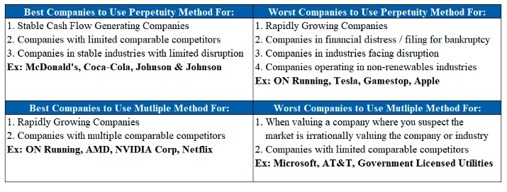
Summary: When to Use Each Method