The Quagmire Challenge: Football Frenzy (April 2018)
The Question
Working in Excel doesn’t always need to be serious. While we typically use Excel to build financial models or data analysis tools, we like to have fun with it from time to time. Over the years, we have built Excel tools for various office pools including The Oscars, March Madness, the NHL Playoffs, fitness challenges, and most importantly for this Quagmire: The FIFA World Cup.
In this challenge, your task is to build a small part of a World Cup predictions tool. In this part of the tool, the user will have to select the top scorers for each of the four teams in one of the World Cup groups of their choosing.
We started you off by compiling each of the countries into their groups as well as assembling rosters for each country according to Wikipedia (official rosters were not available at publishing time). We even created and formatted the table for you (aren’t we nice?). Click here to download the file.

The tool should do the following:
- Allow the user to select which group (A – H) they want to populate the table

- Have the four countries in the group automatically populate (order doesn’t matter) based on the group selected
- Automatically populate each country’s world ranking in the “WR” column
- Hint: the countries are organized by world rank on the “Flags” tab
- Allow the user to predict the rankings of the group at the end of the group stage
- Options are: “1”, “2”, or “Not Advance”

- Options are: “1”, “2”, or “Not Advance”
- Allow the user to select the top scorer for each country based on an automatically created list. The list should be unique for each country, should update depending on which group is selected, and should not contain any extra blank spaces
- Hint: the player lists for each country are included on the “Squads” tab

- Hint: the player lists for each country are included on the “Squads” tab


EXTRA CREDIT: Bonus points to anyone who can outsmart the Quagmire AND also automate the flags to match the countries. Hint: The flags are on the “Flags” tab. We have also included static flags for Group A.
Have fun and good luck. The top solutions will receive a Marquee prize pack and winners will be announced in the June edition of The BenchMarq. Submit your answer to info@marqueegroup.ca, subject: Quagmire #7.
The Solution
The FIFA World Cup soccer tournament begins on June 14th, and with that the office pools are starting to come out. In our April Quagmire we asked participants to put together a small portion of a World Cup office pool template.
As with our past challenges, this Quagmire had multiples ways to solve each step of the problem. We received many “working” solutions. However, in the end we chose submissions that were the most dynamic and at the same time least complicated. The solution presented below is just one of the possible approaches.
Solution Steps:
Task 1 – Populating the Group Name. To fill in the dropdown with the group names, a combination of Data Validation and Custom Number Formatting are needed.
- Create a List of Groups
- In a range of vertical cells, enter the names of the groups (A – H). We used just the letters since it was easier.
- Create a Drop Down List using Data Validation
- ALT + A + V + V (Data > Validation > Data Validation) opens the validation menu
- Under the Settings tab, select “List” under Allow, and for Source select the range of cells created in step #1 above

- Format the Cell
- Since we created our list of groups using just the letters, we need to format the cell so the name will appear as “Group [x]”. If the this you created in step #1 above included “Group” before the letter, you can skip this step
- Custom Number Formatting was used to populate the field as “Group [x]” when someone types in “x” in the cell. This was done by going to the Format Cells menu (CTRL + 1); on the Number tab, under “Custom” we entered the following format: “Group “@


Task 2 – Populating the Group Teams. To automatically fill in the four team names based on the group letter selected, an INDEX/MATCH or OFFSET/MATCH combination could have been used. The key is to modify the MATCH parameter to pull in the first, second, third, and fourth team of the searched group. To solve this step, the helper blue numbers in column B were used, along with the pre-populated list of team names and groups in C10 to D41.
The following formula was built in cell C3 and copied down for all the other teams in range C4:C6:
=INDEX($C$10:$C$41,MATCH($C$2,$D$10:$D$41,0)+$B3-1)

Task 3 – Automatically Populating World Rankings. This was one of the easier steps of the challenge as it simply requires a lookup function to find the World Ranking of each country on the “Flags” worksheet.
An INDEX/MATCH combination (or VLOOKUP function) could have been used in this case in cell F3 and then copied down for cells F4:F6:
=INDEX(Flags!$C$3:$C$202,MATCH(C3,Flags!$D$3:$D$202,0))

Task 4 – Allowing User to Predict Group Rankings. This step required another set of dropdown cells in column D which allow the user to enter 1, 2 or Not Advance for each team. To do this, a Data Validation with a List was used again, with the same steps as in Task 1.
An extra feature that some submission had, though not required, was to check if the user accidently enters 1 or 2 twice (i.e. assumes that two team finish in 2nd place). This could be checked using a COUNTIF on the 1 and 2 entry. If the count is greater than 1 for either, then an error occurs.
An elegant solution that checks all at once is the following formula that can be written in cell D7, at the bottom of the Rank column:
=IF((COUNTIF($D$3:$D$6,1)=1)*(COUNTIF($D$3:$D$6,2)=1)*(COUNTIF($D$3:$D$6,”Not Advance”)=2),””,”You need to select one 1st place team, one 2nd place team, and two teams to not advance”)

Task 5 – Allowing User to Select Top Scorer. This step was the hardest and required a dropdown list for each country that was dynamically populated with the player names for each country. There were many solutions to this task; however, we were looking for the following criteria for a “perfect” answer:
- The solution needed to be dynamic – once it was setup for the first team in cell E3, it should be as easy as copying that cell down three times for the other countries (instead of creating a custom formula for each team)
- The solution needed to be flexible to account for different sized teams – some teams had 30 players in their squad, while others had as few as 22 players; the solution needed to be flexible so that no trailing blank rows would show up in the drop-down menu
- The solution needed to be relatively simple to set up – some solutions we saw used named ranges for each country squad to account for different number of players; this works, however, it takes longer to set up and is also not dynamic (if used in the future as a template, or if the squads change)
Our preferred solution uses either an OFFSET/MATCH or INDEX/MATCH along with a COUNTA to dynamically count how many team players are in each squad. We use this approach when we teach Dynamic Named Ranges in our Advanced Data Manipulation with Excel class to dynamically populate charts, pivot tables and formulas. The formula could either be written directly in the “Source” of the data validation menu or it could be set as a formula of a dynamic named range, and the named range could then be used as the Source.
The following is the step-by-step solution using an OFFSET function.
- With cell E3 selected, insert a new named range: ALT + M + M + D (Formulas > Define Name > Define Name)
- Under Name enter a name for your dynamic named range (e.g. “Players”)
- Under Refers To enter the following OFFSET formula:=OFFSET(Squads!$A$1,1,MATCH(‘Quagmire (Exercise)’!$C3,Squads!$B$1:$AG$1,0), COUNTA(OFFSET(Squads!$A$1,1,MATCH(‘Quagmire (Exercise)’!$C3,Squads!$B$1:$AG$1,0),30,1)),1)

- Once the dynamic named range is set up and while still in cell E3, set up a dropdown list again using data validation (ALT + A + V + V) and under Source write out the dynamic name, e.g. =Players
- Copy cell E3 down to remaining teams


The OFFSET function has 5 parameters, with the last two (height and width) usually optional for normal OFFSET functions, but required for a dynamic named range:
=OFFSET(reference, rows, cols, [height], [width])
- For the cols parameter a MATCH is used to determine the correct column to be used for the squad player names; because the country being looked up in cell C3 has a relative reference, whenever this formula is copied down within the Data Validation, it will keep referring to the corresponding country name
- For the height parameter, a COUNTA function is used to determine the correct length of the squad; within the COUNTA another similar OFFSET function is used that pulls in the entire range of 30 players (including any blanks)
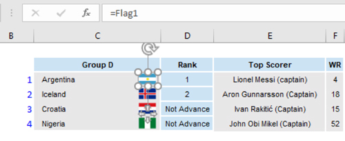
Extra Credit Question: Automating Flags
The easiest way to set this up is to create 4 dynamic named ranges (e.g. “Flag1”, “Flag2”, “Flag3”, “Flag4”), each with its own formula looking up the country names in cells C3, C4, C5, C6. These dynamic named ranges could then be linked up to each picture.
The formulas for the flag named ranges could be either an INDEX/MATCH or OFFSET/MATCH combination again.
The following is the formula for the first flag:
=INDEX( Flags!$E$3:$E$202,MATCH(‘Quagmire (Exercise)’!$C$3,Flags!$D$3:$D$202,0))
The portion that needs to be modified for the other three named ranges is the highlighted “$C$3” (change to $C$4, $C$5, etc.).
To link up the defined name to each picture the following steps should be followed:
- Select the image
- Hit F2 to enter the Formula Bar
- Write out =Flag1 (or Flag2, Flag3, etc.) and hit Enter
If the above INDEX/MATCH function is written inside a regular cell, it will return the contents of the found range. However, when linked up to a picture, it will return whatever is “shown” in that same cell, including any images or shapes on top of the cell. In the example below, the formula will find cell E4 on the Flags worksheet and will return the Argentina flag which is located on top of cell E4.