The Quagmire Challenge: Made to Measure (November 2017)
The Question
Data tables represent one of the quickest and most powerful tools in Excel to measure sensitivities to changes in selected variables. A data table runs in the background constantly (unless your calculation method is set to “Automatic except for data tables”) without affecting your model. Any updates to the model are automatically reflected in the data tables which makes them ideal tools for summary schedules and analysis.
Data tables can be one or two dimensional but how do you handle a sensitivity involving three variables? This very question faces a model builder for Drysdale Oil & Gas – how to handle sensitivities for oil prices, natural gas prices and cost savings in one data table.
If you click here you can download the spreadsheet with the sample data.
The spreadsheet provides a very simple model to determine the EBITDA of Drysdale Oil & Gas.
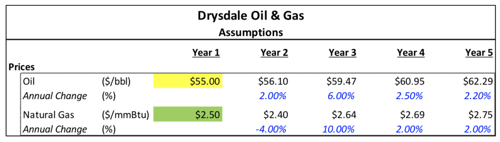
Your task: populate the sensitivity tables outlined in orange.
The first data table will measure three things:
- The change in starting oil price for Year 1 of the forecast period based on the data table inputs ($55.00, $57.50, etc);
- The change in starting gas price for Year 1 of the forecast period based on the data table inputs ($2.50, $2.75, etc); and
- The change in operating annual cost savings (you will have to incorporate an operating annual cost savings into the income statement – assume all years are equal to the first year).
The second data table will measure the percentage increase over the base case EBITDA for each combination of variables in the first data table.
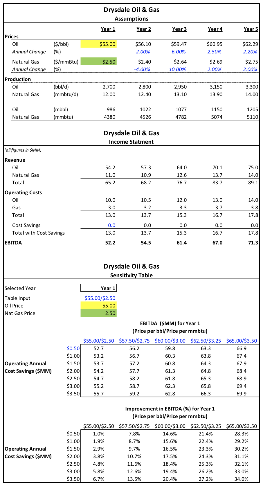
The last feature that the data tables should have is the ability to choose EBITDA from a selected year based on the drop-down list in cell E41.
Have fun and good luck. The top solutions will receive a Marquee prize pack and winners will be announced in the February edition of The BenchMarq. Submit your answer to info@marqueegroup.ca, subject: Quagmire #5.
The Solution
This challenge requires populating two data tables with the added flexibility to choose EBITDA from a selected year based on a drop-down list. Therefore, the solution can be thought of in two parts:
- Data table 1, measuring EBITDA based on a starting Oil Price and Natural Gas price for year 1 and an assumption on operating annual cost savings
- Data table 2, measuring the percentage increase over the base case EBITDA for the combination of variables in Data table 1
Steps for Data Table 1:
1. Incorporate the operating annual cost savings
Insert a cost savings line in the model which will reduce the operating costs when arriving at EBITDA. As per the data provided, the first year will be an input and all subsequent years will be equal to the first year. This will be one of the three variables required for our data table sensitivity.
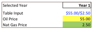
2. Create a Table Input Row to enter the Oil Price and Natural Gas Price for year 1
In order to have a dynamic three variable data table, we inserted three new rows to depict Table Input (row 46), Oil Price (row 47), and Nat Gas Price (row 48) as shown below:
We want the data table to sensitize three variables, but data tables only handle two variables at a time. Keeping in mind our first variable is the operating cost savings, we need to find a way to capture the other two variables (in this case the year 1 Oil Price and Natural Gas Price) in one cell, but allow both variables to feed into the model as drivers.
Excel’s text functions can extract the necessary numbers from the table input cell. We have created an input cell that combines both the Oil Price and the Natural Gas Price in one cell using the format $55.00/$2.50. Since this is a text string and not a number, we have used a simple Mid for the Oil Price and a Right for the Natural Gas Price first to extract the numbers. Then we multiplied by 1 to convert to usable numbers:
Oil Price =MID(E46,2,5)*1 resulting in the number 55.00
Natural Gas Price =RIGHT(E46,4)*1 resulting in the number 2.50
3. Link the Year 1 Oil Price and Natural Gas price in the Assumptions section to the corresponding cells in the inserted rows
The $55.00 seen above is located in cell E7 and linked to the inserted row for Oil Price in year 1 in cell E47. The $2.50 is also linked to the inserted row for Natural Gas cell E48.
4. Enter a formula in the cell located at the intersection of the row and column of input values in Data Table 1
Recall that one of the requirements for this problem was the ability to choose EBITDA from a selected year based on a drop-down list. In order to do this dynamically, the formula utilizes the hlookup function and is as follows for cell D53 in the solution model.=HLOOKUP(E44,$E$5:$I$37,ROWS($E$5:$E$37),FALSE)
This formula assumes:
E44 = the drop-down list with the years
E37 = Row number with EBITDA
5. Highlight the necessary cells for the data table, including the cell at the intersection of the rows and columns (cell D53)
6. Press Alt + A + W + T to bring up the Data Table dialogue box and link the necessary cells for the row and column inputs of our data table

The Row input cell reference is linked to the Table Input and the Column input cell is linked to Cost Savings input.These steps allow us to incorporate both a year 1 Oil and Natural Gas Price in the same cell and then by utilizing Excel’s text functions, convert the text into numbers in cell E47 and E48 which will dynamically link into the model. This allows the ability to sensitize 3 variables in one data table!
We can also change the year in the drop-down box in cell E44 and our EBITDA for that corresponding year will be sensitized based on our inputs.
Steps for Data Table 2:
1. Insert formulas which link to data table 1 in order to determine the percentage increase in EBITDA over the base case (formula should be applied to all cells in data table 2)
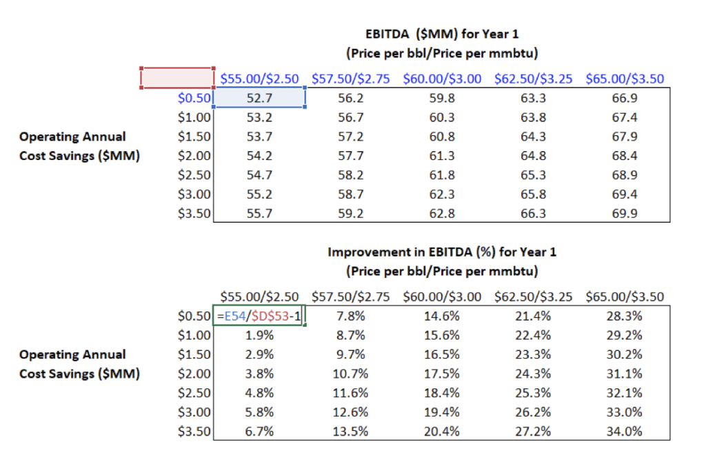
No further work is required to set up Data Table 2. It will now show the percentage increase over the base case EBITDA from a selected year.
Full Model / Solution: